If your SLO says 99.9% but you’ve never actually tested your failover path under sustained load, you don’t have a reliability guarantee – you have a hope. Unplanned downtime costs mid-to-large enterprises upward of $300,000 per hour, according to widely cited industry analyses, yet the majority of reliability gaps surface only after production failures have already burned through error budgets and customer trust. Engineering teams ship faster than ever, but velocity without reliability validation is a liability, not a competitive advantage.
This guide is the unified reliability testing playbook that bridges SRE principles, MTBF metrics, chaos engineering, and load-based availability validation into one executable framework. You’ll move through what reliability testing actually measures (and how it differs from performance testing), how to calculate and operationalize the metrics that matter (MTBF, MTTR, availability percentages, error budgets), how to design test methodologies that expose every failure class from memory leaks to network partitions, and how to prove compliance to stakeholders with reproducible evidence. Every section is built for QA leads, SREs, DevOps managers, and performance engineers who need to act – not just learn definitions.
What Is Reliability Testing? Definition, Scope, and SRE Context
Reliability testing is the systematic validation that a system maintains expected, correct behavior under stress, over extended time horizons, and through deliberate or emergent failure conditions. It answers a fundamentally different question than performance testing: not “how fast?” but “how long, how consistently, and how gracefully does the system recover when something breaks?”
“It’s impossible to manage a service correctly, let alone well, without understanding which behaviors really matter for that service and how to measure and evaluate those behaviors” [1].
Reliability testing is the discipline that generates the empirical evidence behind that understanding.
IEEE formalizes software reliability as “the probability of failure-free software operation for a specified period of time in a specified environment” [2], while ISO 25010 decomposes reliability into four testable sub-characteristics: maturity, availability, fault tolerance, and recoverability [3]. Each of those characteristics maps to a distinct test methodology covered later in this guide.
Reliability Testing vs. Performance Testing: Understanding the Distinction
A load test might confirm your API handles 5,000 requests/second with a p95 latency of 120ms. A reliability test then asks: can it sustain that rate for 48 hours without memory leaking past 85% heap utilization, connection pools draining below 10% available capacity, or p99 latency drifting above 500ms?
Performance testing measures speed and throughput at a point in time. Reliability testing validates that the system maintains correct, consistent behavior across extended time horizons and through failure events. The Google SRE Book’s Chapter 17 (Alex Perry, Max Luebbe) formally separates pre-production test types – unit, integration, system, stress – from production-oriented reliability validation, confirming that reliability testing spans both environments [4]. For a deeper dive into how these different types of performance testing relate to one another, understanding those distinctions helps clarify where reliability validation fits in your overall strategy. Performance is a snapshot; reliability is a time-series.
Both disciplines are necessary. A system that’s fast but unreliable loses users after the third outage in a month. A system that’s reliable but slow never attracts them in the first place. Your test strategy needs both – and the design, duration, and success criteria differ significantly.
SRE Principles and the Role of Error Budgets in Reliability Governance
SRE Team Analyzing Reliability Data
Without SLOs, reliability tests have no pass/fail criteria. Without error budgets, teams have no principled basis for deciding when to freeze releases versus push forward. SRE provides the governance layer that makes reliability testing meaningful.
“The main benefit of an error budget is that it provides a common incentive that allows both product development and SRE to focus on finding the right balance between innovation and reliability. Many products use this control loop to manage release velocity: as long as the system’s SLOs are met, releases can continue” [5].
Here’s how the math works. A service with a 99.9% monthly SLO has an error budget of approximately 43.8 minutes of allowable downtime per 30-day period. If reliability testing in staging consumes simulated “failures” equivalent to 15 minutes of budget, and a production incident burns another 20 minutes in week two, the remaining budget is 8.8 minutes – a signal to halt non-critical deployments and invest in hardening.
“It’s both unrealistic and undesirable to insist that SLOs will be met 100% of the time: doing so can reduce the rate of innovation and deployment, require expensive, overly conservative solutions, or both” [1]. The error budget is a feature, not a flaw – it quantifies the acceptable cost of innovation. Teams looking to formalize their SLA, SLO, and SLI definitions within a performance testing context will find that error budgets become significantly easier to operationalize once these terms are precisely defined.
When Reliability Testing Is Non-Negotiable: Industries and System Types
In financial services, a trading platform outage during market hours can cost millions per minute in lost transactions and regulatory penalties. Basel III operational resilience mandates require institutions to demonstrate they can withstand severe but plausible disruptions – including technology failures – with documented recovery plans. The EU’s Digital Operational Resilience Act (DORA), enforceable since January 2025, explicitly requires financial entities to conduct scenario-based resilience testing of ICT systems, including failover and recovery validation [6].
In healthcare, HIPAA mandates documented disaster recovery plans with defined Recovery Time Objectives (RTO) and Recovery Point Objectives (RPO). An electronic health records system that fails during a critical care workflow doesn’t just violate an SLA – it jeopardizes patient safety.
ISO 25010 codifies reliability as a first-class software quality characteristic [3], and for any system where downtime has financial, safety, or regulatory consequences, reliability testing is a compliance obligation, not an optional engineering practice.
Measuring Reliability: MTBF, MTTR, Availability, and the Metrics That Matter
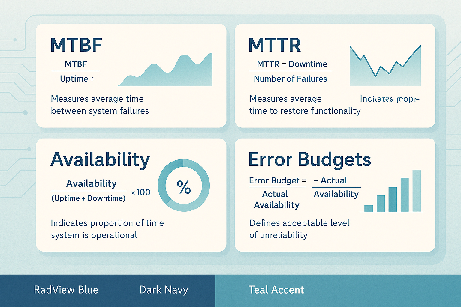
Reliability Testing Metrics Infographic
This section is the one you’ll bookmark. Four metrics form the reliability measurement foundation: MTBF, MTTR, availability percentage, and error budgets. Each has an explicit formula, a concrete interpretation, and a direct connection to SRE governance decisions.
MTBF and MTTR: Formulas, Calculations, and What the Numbers Actually Tell You
MTBF = Total Operational Uptime / Number of Failures
If your web service ran for 2,000 hours over a quarter and experienced 8 incidents requiring remediation, MTBF = 2,000 / 8 = 250 hours. The failure rate (λ) is the inverse: λ = 1/MTBF = 0.004 failures per hour [2].
MTTR = Total Repair Time / Number of Failures
If those 8 incidents required a combined 6 hours of repair time, MTTR = 6 / 8 = 0.75 hours (45 minutes).
IEEE originally developed MTBF for hardware reliability engineering, but the metric requires careful contextualization for software systems [2]. Software failures are rarely random – they cluster around deployments, load spikes, configuration changes, and dependency failures. A raw MTBF of 250 hours means different things depending on whether those failures correlate with release cycles (indicating deployment process issues) or traffic spikes (indicating capacity gaps).
The actionable interpretation: if your MTBF is 250 hours, you’re averaging a failure roughly every 10 days. At 2,500 hours, you’re averaging one every 104 days. The difference between those two numbers often determines whether your team spends its week firefighting or building features – and whether your error budget survives the month.
Availability Percentages, the ‘Nines’ Framework, and Error Budget Calculation
Availability = MTBF / (MTBF + MTTR) × 100
Using the numbers above: 250 / (250 + 0.75) × 100 = 99.70%. Improve MTTR from 45 minutes to 15 minutes (0.25 hours) and availability jumps to 99.90%. This illustrates a crucial insight: reducing repair time is often a faster path to higher availability than reducing failure frequency.
Availability
Annual Downtime
Monthly Error Budget
Typical Use Case
99%
87.6 hours
7.3 hours
Internal tools, batch systems
99.9%
8.76 hours
43.8 minutes
SaaS applications, e-commerce
99.95%
4.38 hours
21.9 minutes
Payment processing, APIs
99.99%
52.6 minutes
4.38 minutes
Financial trading platforms
99.999%
5.26 minutes
26.3 seconds
Core banking, critical infrastructure
As the Google SRE Book states: “It is better to allow an error budget – a rate at which the SLOs can be missed – and track that on a daily or weekly basis” [1]. When your 99.9% service burns 35 of its 43.8 monthly error budget minutes by day 15, that’s the quantitative trigger to pause releases and investigate – not a judgment call, but a data-driven governance decision.
Service Level Indicators (SLIs): Instrumenting Your System to Actually Measure Reliability
SLOs and error budgets are only as good as the SLIs feeding them. An SLI is a specific, measurable quantity that captures a user-visible behavior [1]. The four golden signals from Google SRE practice – latency, traffic, errors, saturation – provide the standard SLI selection framework.
Three concrete SLI specifications your team can implement today:
Availability SLI: Percentage of HTTP requests returning non-5xx responses over a 5-minute rolling window, measured at the load balancer. Target: > 99.9%.
Latency SLI: p99 response time for checkout API calls < 800ms, measured client-side via synthetic probes. Breaches exceeding 2% of requests in a 10-minute window trigger an SLO alert.
Error rate SLI: Ratio of application-level errors (business logic failures, timeout exceptions) to total processed requests, measured at the application instrumentation layer. Target: < 0.1% over a 1-hour window.
Without these instrumented SLIs, MTBF calculations become guesswork and error budget tracking becomes theater. For a broader look at the performance metrics that matter across engineering disciplines, understanding how SLIs connect to throughput, error rates, and resource utilization metrics gives teams a more complete observability picture.
Reliability Testing Methodologies: A Practical Framework From Soak to Failover
Each reliability testing methodology validates a different failure class. The question isn’t “which one should we run?” – it’s “which failure modes can we afford to leave untested?” Google SRE Book Chapter 17 establishes the production test taxonomy spanning stress, canary, and disaster recovery tests [4], and NIST SP 800-160 Vol. 2 provides federal standards guidance for designing systems engineered to withstand disruptions [7].
Failure Mode
Test Methodology
Minimum Duration
Key Metrics to Watch
Memory leak
Endurance/soak test
24 – 72 hours
Heap growth rate, GC frequency
Node failure
Failure injection
Per-scenario (minutes)
Failover time, request error spike
Network partition
Chaos experiment
15 – 60 minutes
Consistency violations, split-brain
Dependency timeout
Circuit breaker test
30 – 60 minutes
Fallback response rate, p99 latency
Disk exhaustion
Soak test with log growth
48+ hours
Disk I/O wait, write error rate
Endurance and Soak Testing: Detecting What Only Time Reveals
Memory leaks, connection pool exhaustion, log file growth consuming disk, and cache hit-ratio degradation are invisible in 30-minute load tests. These failures emerge only after hours or days of continuous operation – exactly the conditions your production system faces. For teams new to this methodology, our dedicated endurance testing in software testing guide provides additional depth on planning and executing extended-duration test runs.
For most production-grade systems, endurance tests should run a minimum of 24 – 72 hours at 70 – 80% of expected peak load. Systems with weekly batch processing cycles should run through at least one full cycle. During execution, monitor three critical indicators continuously:
Heap memory growth rate: A steady upward trend exceeding 2 – 5 MB/hour in a Java service (after accounting for GC cycles) signals a leak that will eventually cause OOM failures.
Active database connections trend: If the connection pool starts at 20/100 active connections and reaches 85/100 after 36 hours without a proportional traffic increase, you have a connection leak.
Disk I/O saturation: Log rotation failures or audit trail accumulation can push disk utilization past 90%, triggering cascading write failures across the application stack.
WebLOAD supports configuring extended-duration load schedules with graduated ramp profiles, enabling teams to simulate realistic diurnal traffic patterns over multi-day test windows while correlating application metrics with infrastructure monitoring data.
Failure Injection and Recovery Testing: Verifying Your Fallback Paths Actually Work
The Principles of Chaos Engineering define the motivation clearly: “We need to identify weaknesses before they manifest in system-wide, aberrant behaviors. Systemic weaknesses could take the form of: improper fallback settings when a service is unavailable; retry storms from improperly tuned timeouts; outages when a downstream dependency receives too much traffic; cascading failures when a single point of failure crashes” [8].
Recovery testing transforms MTTR from an assumed SLA number into a measured outcome. Here’s a concrete test scenario with measurable pass/fail criteria:
Scenario: Terminate the primary database node under 1,000 concurrent users generating mixed read/write workload.
Pass criteria:
Failover to replica completes within 30 seconds
Zero committed transactions lost (RPO = 0)
p99 request latency returns below 500ms within 2 minutes of failover completion
Error rate during failover window does not exceed 2% of total requests
If failover takes 90 seconds instead of 30, that’s 60 seconds of additional MTTR your SLO didn’t account for – and it compounds across every failure event in a month.
NIST SP 800-160 Vol. 2 codifies “Respond” and “Recover” as explicit system resilience functions that must be validated through testing, not assumed through architecture [7].
Redundancy and Distributed Systems Reliability Testing
Distributed architectures introduce failure modes that monoliths never face. The CAP theorem constrains every distributed system to choose between consistency and availability during network partitions – and reliability tests must explicitly validate which trade-off your architecture makes.
Two test scenarios every distributed system needs:
Scenario 1 – Circuit breaker validation: Simulate a network partition between microservice A and its downstream dependency B while under 500 RPS load. Validate that the circuit breaker opens within 5 seconds and the fallback response is served with <200ms latency. If the circuit breaker never opens, you’ll discover during a production outage that your resilience pattern is misconfigured.
Scenario 2 – Database replication under write load: Kill the primary database during active write operations. Validate replica promotion completes within the configured timeout and zero committed transactions are lost. For active-active configurations, verify that conflict resolution handles concurrent writes to both nodes without silent data corruption.
Distributed System with Reliability Patterns
Michael Nygard’s stability patterns – circuit breakers, bulkheads, and timeouts – describe the resilience mechanisms that reliability testing must exercise [9]. Without testing, these patterns are code that has never been proven.
Chaos Engineering and Reliability Testing: Proactive Resilience vs. Reactive Validation
Exploring Chaos in Reliability Testing
Reliability testing validates known system behaviors against defined criteria. Chaos engineering explores unknown failure modes by deliberately inducing turbulent conditions. Both are necessary, but they serve different purposes.
The Principles of Chaos Engineering (Community Standard) defines it precisely: “Chaos Engineering is the discipline of experimenting on a system in order to build confidence in the system’s capability to withstand turbulent conditions in production” [8]. Netflix originated the practice with Chaos Monkey, and Google SRE Book Chapter 17 references both Chaos Monkey and Jepsen as validated production reliability tools [4]. For a practical walkthrough of implementing these principles with real-world examples, our guide on mastering chaos testing covers key learnings and step-by-step execution.
Designing Safe Chaos Experiments: Blast Radius, Hypotheses, and Rollback Plans
Define steady state with specific measurable criteria (e.g., “p99 latency remains below 300ms and error rate stays below 0.1%”).
Hypothesize that steady state will continue in both control and experimental groups.
Inject the failure variable – introduce the real-world event (node crash, network partition, dependency slowdown).
Compare steady-state metrics between control and experimental groups. Disproved hypothesis = discovered weakness.
Before running any experiment, complete this pre-experiment safety checklist:
Steady-state metrics defined and baselined for minimum 24 hours
Blast radius explicitly scoped (percentage of traffic, specific service instance, single availability zone)
Monitoring and alerting confirmed active and validated with a test alert
Rollback procedure documented, tested independently, and executable in < 60 seconds
On-call engineer present during experiment window with kill-switch access
The Principles of Chaos Engineering advocate for production experimentation to get realistic results, but with explicit safeguards. Teams with low chaos maturity should start in staging environments and graduate to production as confidence grows.
Common Chaos Scenarios and What They Reveal
Chaos Scenario
Failure Mode Exposed
Pass Criteria Example
Instance/pod termination
Single point of failure, inadequate auto-scaling
Replacement pod scheduled in < 15s; zero user-facing errors
Network latency injection (200ms added)
Timeout misconfiguration, retry storms
No cascading timeouts; p99 latency increase < 400ms total
Dependency failure (external API returns 503)
Missing fallback logic, tight coupling
Circuit breaker opens in < 5s; graceful degradation response served
CPU exhaustion (90%+ utilization)
Thread pool starvation, priority inversion
Critical path requests still complete within SLO; non-critical traffic shed gracefully
No authentication failures; distributed lock behavior remains correct
Each scenario maps to the systemic weaknesses enumerated in the Principles of Chaos Engineering: “retry storms from improperly tuned timeouts; outages when a downstream dependency receives too much traffic; cascading failures when a single point of failure crashes” [8].
Implementing Reliability Validation With Load Testing
Reliability testing requires sustained, realistic traffic generation – not synthetic spikes. Validating SLOs under production-like conditions means generating multi-protocol load across the full application stack (HTTP, WebSocket, database calls, message queues) for durations measured in hours or days, not minutes.
RadView’s WebLOAD platform supports this with 150+ protocol integrations and the ability to configure multi-day test schedules with graduated load profiles that mirror real diurnal traffic patterns. During endurance runs, WebLOAD’s correlation engine maps application-layer metrics (response time, error rate, throughput) to infrastructure telemetry, enabling teams to pinpoint whether a p99 latency spike at hour 36 is caused by a memory leak, a database connection exhaustion, or an external dependency degradation.
For automated recovery testing, scripted failover scenarios within load test execution allow MTTR measurement under realistic conditions: trigger a node failure at 70% load, measure time-to-recovery, and validate that error rates return within SLO thresholds – all within a single, reproducible test run.
Frequently Asked Questions
How long should reliability tests run to produce actionable results?
The minimum depends on the failure class you’re targeting. Memory leaks and connection pool exhaustion typically require 24 – 72 hours to surface. If your system has weekly batch jobs, cron-triggered maintenance, or periodic cache refreshes, run through at least one full cycle. A common mistake is running soak tests for 8 hours and declaring victory – most production-impacting resource leaks manifest between hours 18 and 48.
Is pursuing 99.999% availability always worth the investment?
Not always. Moving from 99.99% to 99.999% reduces your annual downtime allowance from 52.6 minutes to 5.26 minutes – a 10x reduction that typically requires redundant infrastructure across multiple regions, automated failover with sub-second detection, and near-zero-downtime deployment pipelines. For an internal analytics dashboard, that investment is almost certainly unjustifiable. For a core banking transaction processor, it’s non-negotiable. Let the cost of downtime per minute dictate the target, not engineering ambition.
What’s the most commonly overlooked failure mode in reliability testing?
Gradual resource exhaustion – particularly database connection pool leaks and log-driven disk saturation. These don’t trigger alerts until they cross a threshold, and by that point the system is already in a degraded state. Teams that only run short-duration load tests systematically miss these because the leak rate is often < 1% of the pool per hour, invisible in a 30-minute test window but catastrophic over 72 hours.
How do you get organizational buy-in for chaos engineering when leadership fears production experiments?
Start with data, not philosophy. Run your first chaos experiments in staging against production-like traffic (generated by your load testing platform). Document the failures you discover – misconfigured circuit breakers, missing fallback paths, retry storms – and calculate the cost of those failures if they’d occurred in production. Present the findings as “here’s what we found before our customers did.” Once leadership sees the ROI of proactive discovery, the conversation about controlled production experiments becomes significantly easier.
Reliability metrics (MTBF, availability percentages, error budgets) presented in this guide are illustrative calculations based on generalized models and should be adapted to specific system architectures and operational contexts. Compliance references (DORA, Basel III, HIPAA) reflect general guidance at time of publication and are not legal or regulatory advice – readers should consult qualified compliance professionals for their specific jurisdictions.
References and Authoritative Sources
Jones, C., Wilkes, J., Murphy, N., & Smith, C. (2017). Chapter 4 – Service Level Objectives. In B. Beyer, C. Jones, J. Petoff, & N.R. Murphy (Eds.), Site Reliability Engineering: How Google Runs Production Systems. O’Reilly Media / Google. Retrieved from https://sre.google/sre-book/service-level-objectives/
IEEE. IEEE Standard Glossary of Software Engineering Terminology (IEEE 610.12) and related reliability engineering standards. Institute of Electrical and Electronics Engineers. Referenced for formal definitions of software reliability, MTBF, and failure rate metrics.
ISO/IEC. (2011). ISO/IEC 25010:2011 – Systems and software engineering – Systems and software Quality Requirements and Evaluation (SQuaRE) – System and software quality models. International Organization for Standardization. Referenced for reliability sub-characteristics: maturity, availability, fault tolerance, recoverability.
Perry, A., & Luebbe, M. (2017). Chapter 17 – Testing for Reliability. In B. Beyer, C. Jones, J. Petoff, & N.R. Murphy (Eds.), Site Reliability Engineering: How Google Runs Production Systems. O’Reilly Media / Google. Retrieved from https://sre.google/sre-book/testing-reliability/
Alvidrez, M., & Roth, M. (2017). Chapter 3 – Embracing Risk. In B. Beyer, C. Jones, J. Petoff, & N.R. Murphy (Eds.), Site Reliability Engineering: How Google Runs Production Systems. O’Reilly Media / Google. Retrieved from https://sre.google/sre-book/embracing-risk/
European Union. (2022). Regulation (EU) 2022/2554 – Digital Operational Resilience Act (DORA). Official Journal of the European Union. Referenced for ICT resilience testing requirements applicable to financial entities.
Ross, R., Pillitteri, V., Graubart, R., Bodeau, D., & McQuaid, R. (2021). NIST Special Publication 800-160, Volume 2, Revision 1 – Developing Cyber-Resilient Systems: A Systems Security Engineering Approach. National Institute of Standards and Technology. Retrieved from https://csrc.nist.gov/publications/detail/sp/800-160/vol-2-rev-1/final
Principles of Chaos Engineering. (2019). Principles of Chaos Engineering. Community-maintained reference, originated by Netflix engineering. Retrieved from https://principlesofchaos.org/
Nygard, M.T. (2018). Release It! Design and Deploy Production-Ready Software (2nd ed.). Pragmatic Bookshelf. Referenced for circuit breaker, bulkhead, and timeout stability patterns.
Get a WebLOAD for 30 day free trial. No credit card required.
“WebLOAD Powers Peak Registration”
Webload Gives us the confidence that our Ellucian Software can operate as expected during peak demands of student registration
Steven Zuromski
VP Information Technology
“Great experience with Webload”
Webload excels in performance testing, offering a user-friendly interface and precise results. The technical support team is notably responsive, providing assistance and training
Priya Mirji
Senior Manager
“WebLOAD: Superior to LoadRunner”
As a long-time LoadRunner user, I’ve found Webload to be an exceptional alternative, delivering comparable performance insights at a lower cost and enhancing our product quality.